Controls in Robotics - Robotics Nanodegree by Udacity (Term1)

1. Introduction

Control theory includes:

• open loop controls

1.1 Open loop controls

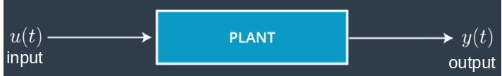
where:

• $u(t)$ input from controller
• Plant is the system to be controlled
• Output ($y(t)$) is the response of the system

1.2 Closed loop control aka feedback

The error between the setpoint value and the current sensor value is sent to the controller.

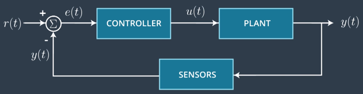
• $r(t)$ reference signal or setpoint
• $e(t)$ is the error signal: $e(t) = r(t) - y(t)$
• $\Sigma$: summing node

The schematic that describes a control system is called a block diagram. The controller takes the error and converts it into a command that is set to the system

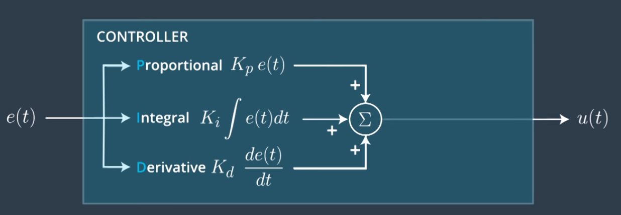
2. PID Controller

The PID controller uses 3 parameters:

• Proportional: $K_p e(t)$
• Integral: $K_i \int e(t) dt$
• Derivative: $K_d \frac{d\ e(t)}{dt}$

where $K_p$, $K_i$, $K_d$ are called gains.

$$\begin{align} \Sigma = K_p e(t) + K_i \int e(t) dt + K_d \frac{d\ e(t)}{dt} \end{align}$$

2.1. Parameters

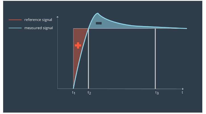
Many real-world systems exhibit a transient oscillatory response to a step input before setting to some steady state value.

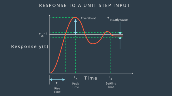
The following components can be tracked when optimizing PID gains optimize

• $T_s$ Steady state offset
• Rise Time
• Maximum percent overshoot: $\begin{align} M_{OS} = \frac{y(T_p) - y(T_{ss})}{y(T_{ss}} \end{align}$

3.2. Effects of PID gains

• Proportional Error: higher $K_p$ results in overshooting and in more oscillations but decrease offset at steady state (SSE=steady state error).
• Integral Error: takes into account accumulated error i.e all past error. It helps eliminate the SSE. If $K_i$ too small tends to correct for the SSE. If $K_i$ is too large, the system becomes unstable.
• Derivative Error: attempts to predict what the error will be by linearly extrapolating the change in error value: $\begin{align} \frac{d \ e(t)}{dt} = \frac{error - lastError}{\Delta t} \end{align}$ Low $K_d$ results in more oscillations and lower rise time. High $K_d$ drives overshoot down, decrease the settling time.

3.3. Limitations of PID

PID does not work well for systems with significant deadtime, lag or higher order dynamics. Dead time is defined as the time before the process variable begins to react to a change in the control output.

3..3.a. Integrator or Integral windup

Integrator windup refers to the situation in a PID feedback controller where a large change in setpoint occurs and the integral terms accumulates a significant error during the rise (windup) thus overshooting and continuing to increase as the accumulated error is unwound.

One way to combat integrator windup is to stop integrating the error if the controller output is saturated.

3.2.b. Disadvantages of Derivative Error

In the presence of high frequency noise, the Derivative Error would increase. A solution is to add a low pass filter to remove some of the high frequency noise, but it can degrades the performance of the derivative control.

A possible low pass filter is First Order recursive filter:

$$\begin{align} \hat{D}[k] = \alpha \frac{e[k] - D[k-1]}{\Delta t} + (1- \alpha) D[k-1] \end{align}$$

where $\alpha \in$ [0,1] is called the smoothing factor. The more $\alpha$ is small, the more high freqeuncy noise are suppressed.

4. Objective of a controller

• Stability: BIBO (bounded input/bounded output), asymptotic stability.
• Tracking refers to the controller’s ability to follow or maintain a reference input signal. The difference between the setpoint and the actual output = tracking error.
• Robustness: Controllers should be valid over a broad range parameter values.
• Disturbance rejection: controllers must be tolerant of disturbances.
• optimality: In many cases, it is important to optimize some property of the system (minimize distance traveled, tracking error). Optimal control requires a mathematical model of the system, constraint equations that set upper/lower limits of the control inputs and a cost function (cost function optimizers includes gradient descent/ascent).

5. TuningStrategies of the Gains

5.1. Manual

• set $K_p$ to small value and $K_i = K_d = 0$
• slowly increase $K_p$ to decrease rise time
• Slowly increase $K_d$ to reduce overshoot and settling time.

5.2 Gradient Descent algorithm aka Twiddle

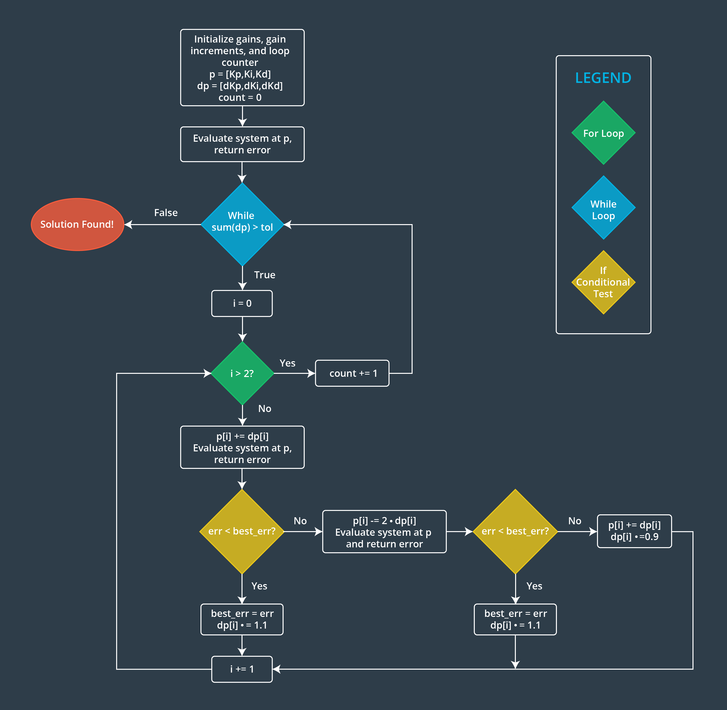
The cost function can be: maximum percent overshoot, settling time, or linear combination.