Derivation of the Gradient of the cross-entropy Loss

Cross-entropy for 2 classes:

$$\begin{align} Xentropy = - \sum_i (y_i log(p_i) ) + (1 - y_i log(1 - p_i)) \end{align}$$

Cross entropy for $c$ classes:

$$\begin{align} Xentropy = - \frac{1}{m} \sum_c \sum_i (y_i ^c log(p_i ^c) ) \end{align}$$

In this post, we derive the gradient of the Cross-Entropy loss $\mathcal{L}$ with respect to the weight $w_{ji}$ linking the last hidden layer to the output layer. Unlike for the Cross-Entropy Loss, there are quite a few posts that work out the derivation of the gradient of the L2 loss (the root mean square error).

When using a Neural Network to perform classification tasks with multiple classes, the Softmax function is typically used to determine the probability distribution, and the Cross-Entropy to evaluate the performance of the model. Then, with the back-propagation algorithm computed from the gradient values of the loss with respect to the fitting parameters (the weights and bias), we can find the optimum parameters that reduces to a minimum the loss between the prediction of the model and the ground truth. For example, the rule update to optimize the weight parameter is:

$$\begin{align} \Delta_{w_{ji}} &= \nabla_{w_{ji}} \mathcal{L} \\ w_{ji} &:= w_{ji} - \alpha \Delta_{w_{ji}} \end{align}$$

Let’s start by rolling out a few definitions:

1. Ground truth is a hot-encoded vector: $y = \left[ \begin{smallmatrix} 0 \\ 0 \\ 1 \\0 \\ .. \\ .. \\ \end{smallmatrix} \right] \in \mathbb{R}^n$ where $n$ is the number of classes (number of rows).

2. Modeled/Predicted probability distribution: $\hat{y} = \left[ \begin{smallmatrix} \hat{y}_0 \\ \hat{y}_1 \\ .. \\ \hat{y}_i \\ .. \\ \end{smallmatrix} \right] \in \mathbb{R}^n$, where the $i$-th element is given by the softmax transfer function.

3. Softmax transfer function: \begin{equation} \hat{y}_i = \frac{e^{z_i}}{\sum_k e^{z_k}} \end{equation} where $z_i = w_{ji} x_j + b_i$ is the $i$-th pre-activation unit. The softmax transfer function is typically used to compute the estimated probability distribution in classification tasks involving multiple classes.

4. The Cross-Entropy loss (for a single example):

$$\mathcal{L} = - \sum_k y_k \ log \ \hat{y}_k$$

Simple model

Let’s consider the simple model sketched below, where the last hidden layer is made of 3 hidden units, and there are only 2 nodes at the output layer. We want to derive the expression of the gradient of the loss with respect to $w_{21}$: $\frac{\partial \mathcal{L}}{\partial w_{21}}$.

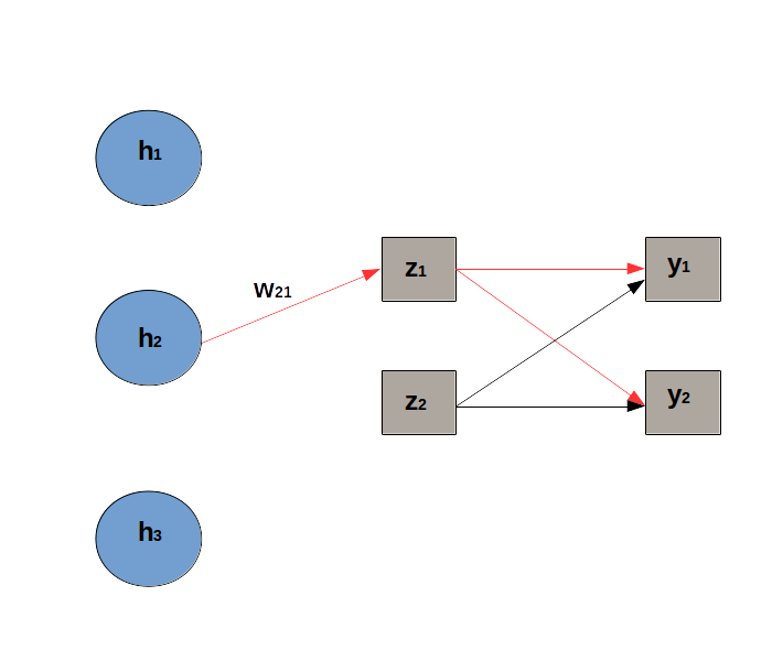
The 2 paths, drawned in red, are linked to $w_{21}$.

The network’s architecture includes:

• a last hidden layer with 3 hidden units.

• The output layer has 2 units to predict the probability distribution with 2 classes.

• $w_{21}$ is the weight linking unit $h_2$ to the pre-activation $z_1$.

• The pre-activation $z_1$ is given by: $\begin{equation} z_1 = h_2 w_{21} + b_2 \end{equation}$

Because, there are 2 paths through $\hat{y}$ that leads to $w_{21}$, we need to sum up the derivatives that go through each path:

$$\begin{align} \frac{\partial \mathcal{L}}{\partial w_{21}} &= \left( \frac{\partial \mathcal{L}}{\partial \hat{y}_1} \frac{\partial \hat{y}_1}{\partial z_1} \frac{\partial z_1}{\partial w_{21}} + \frac{\partial \mathcal{L}}{\partial \hat{y}_2} \frac{\partial \hat{y}_2}{\partial z_1} \frac{\partial z_1}{\partial w_{21}} \right) \\ &= \left( \frac{\partial \mathcal{L}}{\partial \hat{y}_1} \frac{\partial \hat{y}_1}{\partial z_1} + \frac{\partial \mathcal{L}}{\partial \hat{y}_2} \frac{\partial \hat{y}_2}{\partial z_1} \right) \frac{\partial z_1}{\partial w_{21}} \end{align}$$

Let’s calculate the different parts of the equation above:

1. $\frac{\partial z_1}{\partial w_{21}}$

The pre-activation $z_1$ is given by: $z_1 = h_2 w_{21} + b$, hence: $\begin{equation} \frac{\partial z_1}{\partial w_{21}} = h_2 \end{equation}$

2. $\frac{\partial \hat{y}_1}{\partial z_1}$

From the definition of the softmax function, we have $\hat{y_1} = \frac{e^{z_1}}{e^{z_1} + e^{z_2}}$, so:

$$\begin{align} \frac{\partial \hat{y}_1}{\partial z_1} = \frac{\partial}{\partial z_1} \frac{e^{z_1}}{e^{z_1} + e^{z_2}} = \frac{e^{z_1}(e^{z_1} + e^{z_2}) - e^{z_1} e^{z_1}}{(e^{z_1} + e^{z_2})^2} \end{align}$$

We use the following properties of the derivative: $(e^u)' = e^u$ and $\left( \frac{u}{v} \right)' = \frac{u'v - uv'}{v^2}$.

We can then simplify the derivative:

$$\begin{align} \frac{\partial \hat{y}_1}{\partial z_1} = \underbrace{\frac{e^{z_1}}{\left(e^{z_1} + e^{z_2}\right)}}_{\hat{y}_1} - \underbrace{\frac{(e^{z_1})^2}{\left( e^{z_1} + e^{z_2} \right)^2}}_{\hat{y}_1 ^2} \end{align}$$

because $\hat{y}_1 = \frac{e^{z_1}}{e^{z_1} + e^{z_2}}$.

3. $\frac{\partial \hat{y}_2}{\partial z_1}$

Again, from using the definition of the softmax function:

$$\begin{align} \frac{\partial \hat{y}_2}{\partial z_1} = \frac{\partial}{\partial z_1} \frac{e^{z_1}}{e^{z_1} + e^{z_2}} = \frac{0 - e^{z_1} e^{z_2}}{(e^{z_1} + e^{z_2})^2} = - \hat{y}_1 \hat{y}_2 \end{align}$$

4. $\frac{\partial \mathcal{L}}{\partial \hat{y}_{1,2}}$

We start with the definition of the cross-entropy loss: $\mathcal{L} = y_1 \ log \ \hat{y}_1 + y_2 \ log \ \hat{y}_2$:

$$\begin{align} \frac{\partial \mathcal{L} }{\partial \hat{y}_1} = \frac{1}{\hat{y}_1} y_1 + 0 \end{align}$$

and similarly:

$$\begin{align} \frac{\partial \mathcal{L} }{\partial \hat{y}_2} = 0 + \frac{1}{\hat{y}_2} y_2 \end{align}$$

We can now put everything together:

$$\begin{align} \frac{\partial \mathcal{L}}{\partial w_{21}} &= \left( \frac{y_1}{\hat{y}_1} (\hat{y}_1 - \hat{y}_1 ^2) + \frac{y_2}{\hat{y}_2} (-\hat{y}_1 \hat{y}_2) \right) h_2 \\ &= \left( \frac{y_1 \hat{y_1}}{\hat{y}_1} (1 - \hat{y}_1) - y_2 \hat{y}_1 \right) h_2 = \left( y_1 - y_1 \hat{y}_1 - y_2 \hat{y}_1 \right) h_2 \\ &= \left( y_1 - \hat{y}_1 \underbrace{(y_1 + y_2)}_{=1} \right) h_2 \end{align}$$

Hence, finally:

$$\begin{align} \frac{\partial \mathcal{L}}{\partial w_{21}} = (y_1 - \hat{y}_1)h_2 \end{align}$$

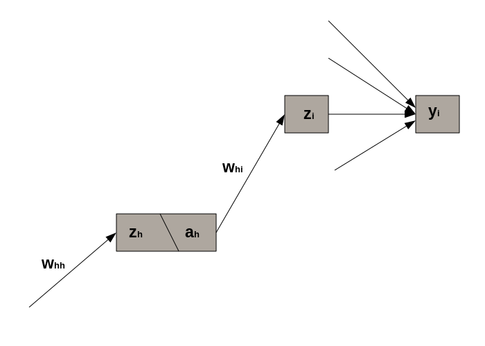
General form of $\frac{\partial \mathcal{L}}{ \partial w_{ji}}$

We start with the definition of the loss function: $\mathcal{L} = -\sum_k y_k \ log \ \hat{y}_k$.

$$\begin{align} \frac{\partial \mathcal{L}}{\partial w_ji} &= \frac{\partial \mathcal{L}}{\partial z_i} \frac{\partial z_i}{\partial w_{ji}} \end{align}$$

From the definition of the pre-activation unit $z_i = h_j w_{ji} + b_j$, we get:

$$\begin{align} \frac{\partial z_i}{\partial w_{ji}} = h_j \end{align}$$

where $h_j$ is the activation of the $j$-th hidden unit.

Now, let’s calculate $\frac{\partial \mathcal{L}}{\partial z_i}$. This term is a bit more tricky to compute because $z_i$ does not only contribute to $\hat{y}_i$ but to all $\hat{y}_k$ because of the normalizing term $\left(\sum_t e^{z-t}\right)$ in $\hat{y}_k = \frac{e^{z}_k}{\sum_t e^{z_t}}$.

Similarly to the toy model discussed earlier, we need to accumulate the gradients wrt $z_i$ from all relevant paths.

$$\begin{align} \frac{\partial \mathcal{L}}{\partial z_i} = \frac{\partial \mathcal{L}}{\partial \hat{y}_i} \frac{\partial \hat{y}_i}{\partial z_i} + \sum_{t \neq i} \frac{\partial \mathcal{L}}{\partial \hat{y}_t} \frac{\partial \hat{y}_t}{\partial z_i} \end{align}$$

The gradient of the loss with respect to the output $\hat{y}_i$ is:

$$\begin{align} \frac{\partial \mathcal{L}}{\partial \hat{y}_i} &= \frac{\partial }{\partial \hat{y}_i} \left(- \sum_u y_u \ log \ \hat{y}_u \right) = -\frac{y_i}{\hat{y}_i} \end{align}$$

Hence:

$$\begin{align} \frac{\partial \mathcal{L}}{\partial z_i} = -\frac{y_i}{\hat{y}_i} \frac{\partial \hat{y}_i}{\partial z_i} + \sum_{t \neq i} \frac{-y_t}{\partial \hat{y}_t} \frac{\partial \hat{y}_t}{\partial z_i} \end{align}$$

The next step is to calculate the other partial derivative terms:

$$\begin{align} \frac{\partial \hat{y}_i}{\partial z_i} = \frac{\partial}{\partial z_i} \frac{e^{z_i}}{\sum_u e^{z_u}} = \frac{e^{z_i} \sum_u e^{z_u} - e^{z_i} e^{z_i}}{(\sum_u e^{z_u})^2} = \underbrace{\frac{e^{z_i}}{\sum_u e^{z_u}}}_{\hat{y}_i} - \underbrace{\left(\frac{e^{z_i}}{\sum_u e^{z_u}}\right)^2}_{\hat{y}_i ^2} = \hat{y}_i - \hat{y}_i ^2 \end{align}$$ $$\begin{align} \frac{\partial \hat{y}_t}{\partial z_i} = \frac{\partial}{\partial z_i} \frac{e^{z_t}}{\sum_u e^{z_u}} = \frac{0 - e^{z_t} e^{z_i}}{(\sum_u e^{z_u})^2} = -\underbrace{\frac{e^{z_t}}{\sum_u e^{z_u}}}_{\hat{y}_t} \ \underbrace{\frac{e^{z_i}}{\sum_u e^{z_u}}}_{\hat{y}_i} = -\hat{y}_t \ \hat{y}_i \end{align}$$

Let’s replace the results above:

$$\begin{align} \frac{\partial \mathcal{L}}{\partial z_i} &= -\frac{y_i}{\hat{y}_i} \hat{y}_i (1 - \hat{y}_i) + \sum_{t \neq i} -\frac{y_t}{\hat{y}_t} (- \hat{y}_t \hat{y}_i) = -y_i + y_i \hat{y}_i + \sum_{t \neq i} y_t \hat{y_i} \\ &= -y_i + \sum_t y_t \hat{y}_i = \hat{y}_i \underbrace{\sum_t y_t}_{=1} - y_i \end{align}$$

Finally, we get the gradient wrt $w_{ji}$

$$\begin{align} \frac{\partial \mathcal{L}}{\partial w_{ji}} = h_j (\hat{y}_i - y_i) \end{align}$$