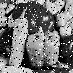
Methods to remove salt and pepper noise
Opening
First cv2.erosion() is applied to get rid of noise and shrinks the object. Then cv2.dilation() enlarges the object back to its original size, or close.
import cv2
import matplotlib.pyplot as plt
import numpy as np

# open image as grayscale
gray = cv2.imread("img.png", 0)

#create a 5x5 kernels of ones
kernel = np.ones((3,3))

dilation = cv2.dilate(gray, kernel, iterations=1)
erosion = cv2.erode(gray, kernel, iterations=1)

#opening: erosion -dilation
opening = cv2.morphologyEx(gray, cv2.MORPH_OPEN, kernel)

plt.figure(figsize=(10, 5))
plt.subplot(121)
plt.title("Original Image - Grayscale")
plt.imshow(gray, cmap="gray")
plt.axis("off")

plt.subplot(122)
plt.title("Opening")
plt.imshow(opening, cmap="gray")
plt.axis("off")
plt.show()

Close
The process is reversed to the opening process.
import cv2
import matplotlib.pyplot as plt
import numpy as np

# open image as grayscale
gray = cv2.imread("img.png", 0)

#create a 5x5 kernels of ones
kernel = np.ones((3,3))

#opening: erosion -dilation
opening = cv2.morphologyEx(gray, cv2.MORPH_CLOSE, kernel)

plt.figure(figsize=(10, 5))
plt.subplot(121)
plt.title("Original Image - Grayscale")
plt.imshow(gray, cmap="gray")
plt.axis("off")

plt.subplot(122)
plt.title("Opening")
plt.imshow(closing, cmap="gray")
plt.axis("off")
plt.show()

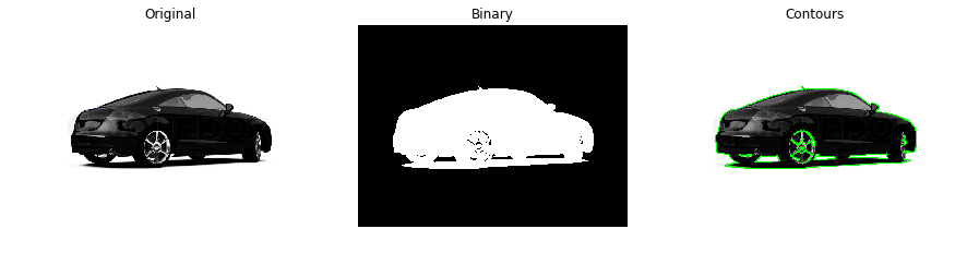
Image Segmentation
Using image contouring is a technique useful for image segmentation: countour is a continuous curve that follows the edges along a boundary.
In openCV, contours are better detected when there is a white object against a black background.
import cv2
import matplotlib.pyplot as plt
import numpy as np

# open image as rgb
original = cv2.imread("car.jpg")
#open image as grayscale
gray = cv2.imread("car.jpg", 0)
# Transform image to binary with threshold
retval, binary = cv2.threshold(gray, 225, 255, cv2.THRESH_BINARY_INV)

"""
Find countours
 :RETR_TREE: contour retrieval mode as a Tree
 :CHAIN_APPROX_SIMPLE: contour approximation method

output
 :contours: list of contours
 :hierarchy: is used if there are many contours nested in one another. The hierarchy defines their relationship
             to one another
"""
retval, contours, hierarchy = cv2.findContours(binary, cv2.RETR_TREE, cv2.CHAIN_APPROX_SIMPLE)

"""Draw contours on a copy of original image

Draw contours on a copy of original image
 :-1: which contour to show (-1 == all)
 :(0, 255, 0): the color
 :2: the pixel width of the contour
"""
original_copy = np.copy(original)
all_contours = cv2.drawContours(original_copy, contours, -1, (0, 255, 0), 2)
Contour features
Contour features are :
- area
- center
- perimeter
- bounding rectangle
Orientation of a contour
To find the orientaion of a contour, the contour is fit to an ellipse:
(x, y), (MA, ma), angle = cv2.fitEllipse(selected_contour)
Bounding rectangle
x, y, w, h = cv2.boundingRect(contour)
K-means for segmentation
# Reshape image into a 2D array of pixels and 3 color values (RGB)
pixel_vals = image.reshape((-1,3))

# Convert to float type
pixel_vals = np.float32(pixel_vals)

#Implement Kmeans in opencv
# define stopping criteria
# you can change the number of max iterations for faster convergence!
criteria = (cv2.TERM_CRITERIA_EPS + cv2.TERM_CRITERIA_MAX_ITER, 100, 0.2)

"""
:k: elect the number of centroids
:None: labels if any
:criteria: stop criteria
:10: number of iterations
:cv2.KMEANS_RANDOM_CENTERS: initialization of the centroid

"""
# then perform k-means clustering
k = 3
retval, labels, centers = cv2.kmeans(pixel_vals, k, None, criteria, 10, cv2.KMEANS_RANDOM_CENTERS)

# convert data into 8-bit values
centers = np.uint8(centers)
segmented_data = centers[labels.flatten()]

# reshape data into the original image dimensions
segmented_image = segmented_data.reshape((image.shape))
labels_reshape = labels.reshape(image.shape[0], image.shape[1])

plt.imshow(segmented_image)