
In this post, I will present a method to reconstruct the input x from an output y and using the trained weight W and trained bias b. We consider a linear activation, with a forward pass:
Motivations
One of the motivations for reconstructing an input x is to get more insights on the internal representation of a Neural Network. For example, it would be interesting to know:
- what input value would shut down a hidden unit?
- how sensitive is the output to the input?
For the sake of demonstrating the concept, I will be using a very simple linear model: a single output and no hidden layers. Nevertheless, the approach could be extended in more complex models, specifically RNN, LSTM. In LSTM for example, one could use the approach to get a better understanding of what type of input shuts down a unit of the forget gate for instance.
Details of the input reconstruction
We start by training the model and then extract the optimized variables W (weights) and b (bias). Instead of predicting the output y0 from x0, we attempt to predict what value x0 must be set to for the model to output y0:
-
We initialize
x0to:x0=1(actually you could use any values, except 0) -
We compute the forward pass:
- As we stated earlier,
Wandbare fixed parameters. Onlyx0is a fitting parameter in the model. We compute how the cost function, which quantifies how far our calculatedypredvalue is from the expectedy0value when usingx0=1
- We then calculate the gradient with respect to the input .
- We can then update the value of
x0using the gradient and a learning ratelr:
The proess can be re-iterated until ypred is close enough to y0.
Demo
For the full code, check out the notebook file here.
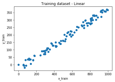
Let’s generate the dataset
#Build dataset
x_train = np.random.uniform(low=0, high=1000, size=(100, 1))
y_train = np.array([0.4 * i -50 * np.random.random() for i in x_train])

#Visualize data
plt.scatter(x_train, y_train)
plt.title("Training dataset - Linear")
plt.xlabel("x_train")
plt.ylabel("y_train")
plt.show()
Train the model
#Train the a simple model to fit the dataset and extract W and bias

model = Sequential()
model.add(Dense(units=1, input_shape=(1, )) )
# now the model will take as input arrays of shape (*, 1)
# and output arrays of shape (*, 1)
model.compile(loss="mse", optimizer="adam")
model.fit(x_train, y_train, epochs=100000, batch_size=100, verbose=0)
model.summary()
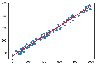
The red line is the best fit using the optimizede weight and bias values.
Reconstruct input x0for output y0=100
Let’s reconstruct the input x0 that would result in an output y0=100. I use a learning rate of 0.2. It is kept constant for during training.
def total_loss(y_mod, y_pred):
    cost_ = K.square(y_mod - y_pred)
    return cost_

x = np.array([1.])
x = x.reshape( (1, 1) )
w = weight.reshape((1, 1))
bias = bias.reshape((1, 1))
y0 = np.array([[100.]])
x_tensor = tf.convert_to_tensor(x, np.float32)
w_tensor = tf.convert_to_tensor(w, np.float32)
b_tensor = tf.convert_to_tensor(bias, np.float32)

y0_tensor = tf.convert_to_tensor(y0, np.float32 )
x_summary = []
n_iter = 200
for iteration in range(n_iter):
    y_pred = K.dot(x_tensor, w_tensor) + b_tensor
    cost_ = total_loss(y0_tensor, y_pred)
    grads = K.gradients(cost_, x_tensor)[0]
    loss = K.mean(cost_)
    lr = K.variable(0.4)
    x_tensor -= lr * grads
    x_summary.append(K.get_value(x_tensor)[0,0])
    if (iteration % 5 == 0) or (iteration==n_iter-1):
        print("Iteration: {} | x value: {}".format(iteration, K.get_value(x_tensor)))

    x0 =  K.get_value(x_tensor)[0, 0]
plt.scatter( np.arange(0, n_iter, 1 ), x_summary)
plt.show()
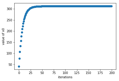
The y-axis is the value of x0 as the number of iterations increases. At high iterations, x0 saturates towards the optimum value of x0=312.
In brief, in order to get an output y0=100, the input must be x0=312.
Let’s see where this points (orange dot) lands on the plot that shows the dataset and of the best fit:
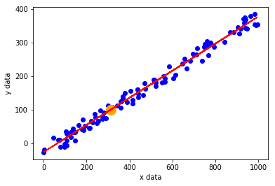
Nice!!! We can now reconstruct the input from the output of a any hidden unit.
Note that I consider a simple case of linear activation.
Adding non-linear activation
Let’s consider the case of the sigmoid function, defined as:
where z = W.x +b.