
In this post, we will identify customers segments using data collected from customers of a wholesale distributor in Lisbon (Portugal). The dataset includes the various customers annual spending amounts (reported in monetary units) of diverse product categories for internal structure. The project includes several steps: explore data (determine if any product categories are highly correlated), scale each product category, identify and remove outliers, dimension reduction using PCA, implement a clustering algorithm to segment the customer data and finally compare segmentation. The dataset for this project can be found on the UCI Machine Learning Repository. For the purposes of this project, the features 'Channel' and 'Region' will be excluded in the analysis — with focus instead on the six product categories recorded for customers.
Let’s load the dataset along with a few of the necessary Python libraries.
Wholesale customers dataset has 440 samples with 6 features each.
Data Exploration
In this section, we begin exploring the data through visualizations to understand how each feature is related to the others. We will observe a statistical description of the dataset, consider the relevance of each feature, and select a few sample data points from the dataset which you will track through the course of this project.
| Fresh | Milk | Grocery | Frozen | Detergents_Paper | Delicatessen | |
| count | 440.000000 | 440.000000 | 440.000000 | 440.000000 | 440.000000 | 440.000000 |
| mean | 12000.297727 | 5796.265909 | 7951.277273 | 3071.931818 | 2881.493182 | 1524.870455 |
| std | 12647.328865 | 7380.377175 | 9503.162829 | 4854.673333 | 4767.854448 | 2820.105937 |
| min | 3.000000 | 55.000000 | 3.000000 | 25.000000 | 3.000000 | 3.000000 |
| 25% | 3127.750000 | 1533.000000 | 2153.000000 | 742.250000 | 256.750000 | 408.250000 |
| 50% | 8504.000000 | 3627.000000 | 4755.500000 | 1526.000000 | 816.500000 | 965.500000 |
| 75% | 16933.750000 | 7190.250000 | 10655.750000 | 3554.250000 | 3922.000000 | 1820.250000 |
| max | 112151.000000 | 73498.000000 | 92780.000000 | 60869.000000 | 40827.000000 | 47943.000000 |
Product Categories - Here are possible products that may be purchased within the 6 product categories:
- Fresh: fruits, vegetables, fish, meat
- Milk: dairy products i.e Milk, cheese, cream
- Grocery: flour, rice, cereals, beverages, can food
- Frozen: frozen vegetables, processed food
- Detergents_paper: household products, Detergent, hand/floor soap, napkins
- Delicatessen: fine chocolate, french cheese
The integer represents the annual spending of a customer in monetary unit (mu) for a particular product category.
Implementation: Selecting Samples
To get a better understanding of the customers and how their data will transform through the analysis, it would be best to select a few sample data points and explore them in more detail.
Chosen samples of wholesale customers dataset:
| Fresh | Milk | Grocery | Frozen | Detergents_Paper | Delicatessen | |
| 0 | 12126 | 3199 | 6975 | 480 | 3140 | 545 |
|---|---|---|---|---|---|---|
| 1 | 4155 | 367 | 1390 | 2306 | 86 | 130 |
| 2 | 17360 | 6200 | 9694 | 1293 | 3620 | 1721 |
| Fresh | Milk | Grocery | Frozen | Detergents_Paper | Delicatessen | |
| 0 | 126.0 | -2597.0 | -976.0 | -2592.0 | 259.0 | -980.0 |
|---|---|---|---|---|---|---|
| 1 | -7845.0 | -5429.0 | -6561.0 | -766.0 | -2795.0 | -1395.0 |
| 2 | 5360.0 | 404.0 | 1743.0 | -1779.0 | 739.0 | 196.0 |
| Fresh | Milk | Grocery | Frozen | Detergents_Paper | Delicatessen | |
| 0 | 3622.0 | -428.0 | 2219.0 | -1046.0 | 2324.0 | -421.0 |
|---|---|---|---|---|---|---|
| 1 | -4349.0 | -3260.0 | -3366.0 | 780.0 | -730.0 | -836.0 |
| 2 | 8856.0 | 2573.0 | 4938.0 | -233.0 | 2804.0 | 755.0 |
[+] customer0’s spending on Milk, Frozen and Delicatessen is lower than the median, but it spends more on Fresh, Grocery and Detergents.
[+] customer1’s spending is lower than the median and the mean for all categories except for ‘Frozen’, for which speding is higher than median but lower than the mean.
[+] customer2 spending is higher than the mean and median spending for all categories except for ‘Frozen’.
The table below details the total spending of each sample customer and the percentage of spending per product categories (‘%cost_’)
| Customer | total cost | %cost_Fresh | %cost_Milk | %cost_Grocery | %cost_Frozen | %cost_Detergents_Paper | %cost_Delicatessen | |
| 0 | 26465 | 45.8 | 12.1 | 26.4 | 1.8 | 11.9 | 2.1 | |
|---|---|---|---|---|---|---|---|---|
| 1 | 8434 | 49.3 | 4.4 | 16.5 | 27.3 | 1.0 | 1.5 | |
| 2 | 39888 | 43.5 | 15.5 | 24.3 | 3.2 | 9.1 | 4.3 |
[+] All the 3 customers purchase mainly ‘Fresh’ products, which accounts for about 50% of their total spending.
[+] Customer0 and Customer2 are likely to be operating in the same business segment, with similar purchase pattern.
Indeed, their 2nd largest expenditure is for ‘Grocery’ products followed by ‘Fresh’ and ‘Frozen’ products.
Customer2 out-spends Customer0 by about 13000mu: that infers that Customer2 may be a larger business and may need more volume. Customer0 and Customer2 may be in the Retail segment, where food related items (Fresh, Milk, Grocery) are typically available, as well as Household products.
[+] For Customer1, the 2nd largest spending is for ‘Frozen’ products followed by ‘Grocery’ products.
Customer1 might be in the Restaurant segment, where the highest percentage of expenditures are for food related items, and the smallest percentage of expenditure for ‘Detergents_Paper’ products. Note also that Customer1 has the smallest total expenditure compared to the 2 other customers, about 3 to 5 times lower than Customer0 and Customer2 respectively. It is very likely that a Restaurant needs less volume than retailers.
As a side note, it might be useful to look at the volume of the purchase for the different product categories to get more insight on the customer business segment. Indeed, ‘Detergents_paper’ products are typically more expensive than ‘Milk’ products for example. Therefore, a larger percentage of expenditure on ‘Detergents_Paper’ does not necessarily mean that the customer purchase a higher volume of ‘Detergents_Paper’ products.
Implementation: Feature Relevance
One interesting thought to consider is if one (or more) of the six product categories is actually relevant for understanding customer purchasing. That is to say, is it possible to determine whether customers purchasing some amount of one category of products will necessarily purchase some proportional amount of another category of products? We can make this determination quite easily by training a supervised regression learner on a subset of the data with one feature removed, and then score how well that model can predict the removed feature.
[+] Deleted feature: Fresh
| Feature importance | |
| Milk | 0.226778 |
|---|---|
| Grocery | 0.082826 |
| Frozen | 0.305044 |
| Detergents Paper | 0.139340 |
| Delicatessen | 0.246012 |
[+] Deleted feature: Milk
| Feature importance | |
| Fresh | 0.138434 |
|---|---|
| Grocery | 0.219012 |
| Frozen | 0.031806 |
| Detergents Paper | 0.465780 |
| Delicatessen | 0.144969 |
[+] Deleted feature: Grocery
| Feature importance | |
| Fresh | 0.020446 |
|---|---|
| Milk | 0.045690< |
| Frozen | 0.016514 |
| Detergents Paper | 0.890934 |
| Delicatessen | 0.026416 |
[+] Deleted feature: Frozen
| Feature importance | |
| Fresh | .098081 |
|---|---|
| Milk | 0.067566 |
| Grocery | 0.064459 |
| Detergents Paper | 0.127549 |
| Delicatessen | 0.642346 |
[+]Deleted feature: Detergents_Paper
| Feature importance | |
| Fresh | 0.040617 |
|---|---|
| Milk | 0.013689 |
| Grocery | 0.900611 |
| Frozen | 0.021572 |
| Delicatessen | 0.023511 |
[+] Deleted feature: Delicatessen
| Feature importance | |
| Fresh | 0.148177 |
|---|---|
| Milk | 0.147138 |
| Grocery | 0.073654 |
| Frozen | 0.487107 |
| Detergents_Paper | 0.143924 |
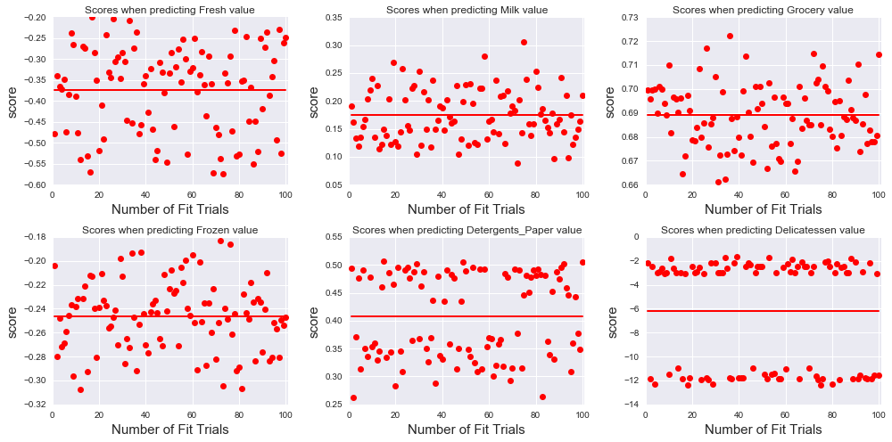
The code above is generalized to study how the score varies when trying to predict any of the 6 attributes. In order to visualize the consistency of the test score values for each case, we run the Decision Tree Regressor multiple times (nbr_fit_trials=100) on the training set and calculate the score of the model on the test set.
The score is defined by:
where is the true value of , is the predicted value, and is the mean of the true value. can be positive with best value of 1. It can also be negative if the model fails to fit the data, i.e if is large.
We obtain a negative score when attempting to predict the values of the feature ‘Milk’ using the 5 other features. Although the score values are scattered for the 100 fit trials , it is consistently negative (the red bar in the plot shows the mean value of the score). Therefore, ‘Milk’ cannot be predicted using the 5 other features and is therefore necessary for identifying customers’ spending habits. Similarly, the values of the features ‘Frozen’ and ‘Delicatessen’ cannot be predicted.
The best average score is obtained when predicting ‘Grocery’ : . This means that, if given the 5 other features, the values of ‘Grocery’ can be determined with relatively good accuracy. Therefore, the feature ‘Grocery’ might not be necessary for identifying patterns in customers’ spending. To a lesser extent, the values of ‘Detergent_papers’ can also be predicted from the remaining features: in this case is close to 50%.
The parameter feature_importance also provides some additional information on the possible correlation between the features, in particular for the 2 cases where is positive.
The importance of a feature is computed as the (normalized) total reduction of the criterion brought by that feature. >It is also known as the Gini importance. Ref. sklearn documentation
When using ‘Grocery’ as the label, the most important feature is ‘Detergent_papers’, with a Gini importance of 0.89, and inversely when using ‘Detergent_papers’ as the label, the feature ‘Grocery’ becomes the most important with a Gini importance of 0.90. The result indicates that there is some correlation between the attribute ‘Grocery’ and ‘Detergent_papers’, although we cannot deduce whether it is a positive or a negative correlation.
Visualize Feature Distributions
To get a better understanding of the dataset, we can construct a scatter matrix of each of the six product features present in the data.
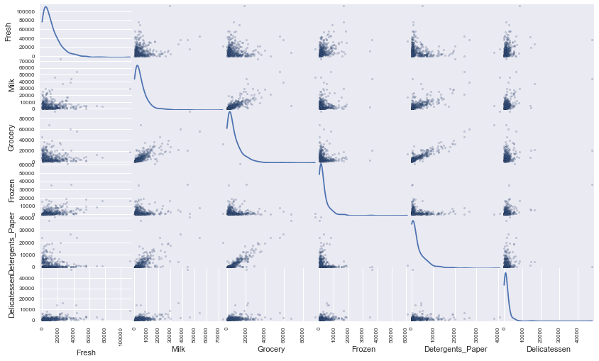
[+] Most features are uncorrelated, except for ‘Grocery’ and ‘Detergents_paper’ which are positively correlated. ‘Grocery’ spending clearly increases with ‘Detergent_paper’ spending. Thus, the values of the feature ‘Grocery’ can be predicted given the values of ‘Detergents_paper’, and vice-versa. There is also evidence of some correlation between other pairs of features: ‘Detergent_papers’ versus ‘Milk’, and ‘Grocery’ versus ‘Milk’, which are all positive correlation. All the 6 attributes show a lognormal distribution (the data is not normally distributed). The distributions are skewed to the right with a long tail: the bulk of the customers have relatively small spending but a few customers have spending much larger.
Data Preprocessing
In this section, we will preprocess the data to create a better representation of customers by performing a scaling on the data and detecting (and optionally removing) outliers. If data is not normally distributed, especially if the mean and median vary significantly (indicating a large skew), it is most often appropriate to apply a non-linear scaling — particularly for financial data. One way to achieve this scaling is by using a Box-Cox test, which calculates the best power transformation of the data that reduces skewness. A simpler approach which can work in most cases would be applying the natural logarithm.
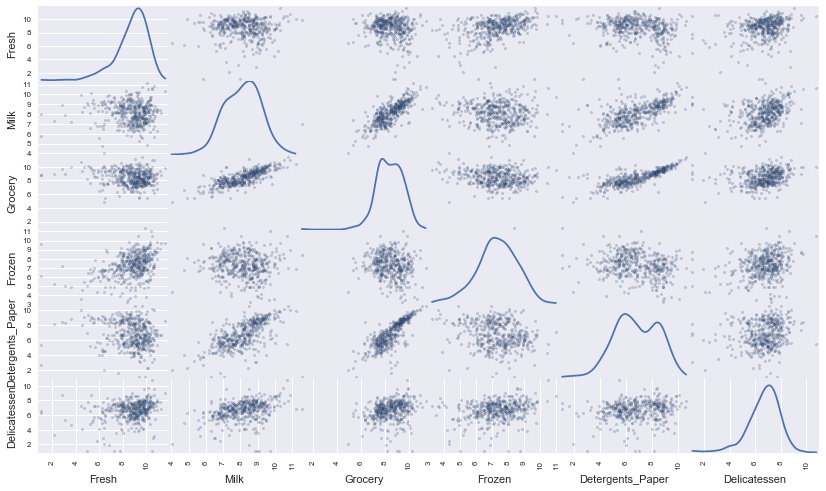
The Log transformation is usually performed on skewed data to make it approximately normal, and that make the transformed data more appropriate to be used with models that assume a normal distribution, like Gaussian Mixture Model. After the transformation of the data, we see a clearer correlation between ‘Detergent_papers’ and ‘Grocery’, and also between ‘Milk’ and ‘Detergent_papers’, and ‘Grocery’ and ‘Milk’.
Run the code below to see how the sample data has changed after having the natural logarithm applied to it.
| Fresh | Milk | Grocery | Frozen | Detergents_Paper | Delicatessen | |
|---|---|---|---|---|---|---|
| 0 | 9.403107 | 8.070594 | 8.850088 | 6.173786 | 8.051978 | 6.300786 |
| 1 | 8.332068 | 5.905362 | 7.237059 | 7.743270 | 4.454347 | 4.867534 |
| 2 | 9.761924 | 8.732305 | 9.179262 | 7.164720 | 8.194229 | 7.450661 |
Implementation: Outlier Detection
Detecting outliers in the data is extremely important in the data preprocessing step of any analysis. The presence of outliers can often skew results which take into consideration these data points. There are many “rules of thumb” for what constitutes an outlier in a dataset. Here, we will use Tukey’s Method for identfying outliers: An outlier step is calculated as 1.5 times the interquartile range (IQR). A data point with a feature that is beyond an outlier step outside of the IQR for that feature is considered abnormal.
[+] Data points considered outliers for the feature ‘Fresh’:
| Fresh | Milk | Grocery | Frozen | Detergents_Paper | Delicatessen | |
|---|---|---|---|---|---|---|
| 65 | 4.442651 | 9.950323 | 10.732651 | 3.583519 | 10.095388 | 7.260523 |
| 66 | 2.197225 | 7.335634 | 8.911530 | 5.164786 | 8.151333 | 3.295837 |
| 81 | 5.389072 | 9.163249 | 9.575192 | 5.645447 | 8.964184 | 5.049856 |
| 95 | 1.098612 | 7.979339 | 8.740657 | 6.086775 | 5.407172 | 6.563856 |
| 96 | 3.135494 | 7.869402 | 9.001839 | 4.976734 | 8.262043 | 5.379897 |
| 128 | 4.941642 | 9.087834 | 8.248791 | 4.955827 | 6.967909 | 1.098612 |
| 171 | 5.298317 | 10.160530 | 9.894245 | 6.478510 | 9.079434 | 8.740337 |
| 193 | 5.192957 | 8.156223 | 9.917982 | 6.865891 | 8.633731 | 6.501290 |
| 218 | 2.890372 | 8.923191 | 9.629380 | 7.158514 | 8.475746 | 8.759669 |
| 304 | 5.081404 | 8.917311 | 10.117510 | 6.424869 | 9.374413 | 7.787382 |
| 305 | 5.493061 | 9.468001 | 9.088399 | 6.683361 | 8.271037 | 5.351858 |
| 338 | 1.098612 | 5.808142 | 8.856661 | 9.655090 | 2.708050 | 6.309918 |
| 353 | 4.762174 | 8.742574 | 9.961898 | 5.429346 | 9.069007 | 7.013016 |
| 355 | 5.247024 | 6.588926 | 7.606885 | 5.501258 | 5.214936 | 4.844187 |
| 357 | 3.610918 | 7.150701 | 10.011086 | 4.919981 | 8.816853 | 4.700480 |
| 412 | 4.574711 | 8.190077 | 9.425452 | 4.584967 | 7.996317 | 4.127134 |
[+]Data points considered outliers for the feature ‘Milk’:
| Fresh | Milk | Grocery | Frozen | Detergents_Paper | Delicatessen | |
|---|---|---|---|---|---|---|
| 86 | 10.039983 | 11.205013 | 10.377047 | 6.894670 | 9.906981 | 6.805723 |
| 98 | 6.220590 | 4.718499 | 6.656727 | 6.796824 | 4.025352 | 4.882802 |
| 154 | 6.432940 | 4.007333 | 4.919981 | 4.317488 | 1.945910 | 2.079442 |
| 356 | 10.029503 | 4.897840 | 5.384495 | 8.057377 | 2.197225 | 6.306275 |
[+] Data points considered outliers for the feature ‘Grocery’:
| Fresh | Milk | Grocery | Frozen | Detergents_Paper | Delicatessen | |
|---|---|---|---|---|---|---|
| 75 | 9.923192 | 7.036148 | 1.098612 | 8.390949 | 1.098612 | 6.882437 |
| 154 | 6.432940 | 4.007333 | 4.919981 | 4.317488 | 1.945910 | 2.079442 |
[+] Data points considered outliers for the feature ‘Frozen’:
| Fresh | Milk | Grocery | Frozen | Detergents_Paper | Delicatessen | |
|---|---|---|---|---|---|---|
| 38 | 8.431853 | 9.663261 | 9.723703 | 3.496508 | 8.847360 | 6.070738 |
| 57 | 8.597297 | 9.203618 | 9.257892 | 3.637586 | 8.932213 | 7.156177 |
| 65 | 4.442651 | 9.950323 | 10.732651 | 3.583519 | 10.095388 | 7.260523 |
| 145 | 10.000569 | 9.034080 | 10.457143 | 3.737670 | 9.440738 | 8.396155 |
| 175 | 7.759187 | 8.967632 | 9.382106 | 3.951244 | 8.341887 | 7.436617 |
| 264 | 6.978214 | 9.177714 | 9.645041 | 4.110874 | 8.696176 | 7.142827 |
| 325 | 10.395650 | 9.728181 | 9.519735 | 11.016479 | 7.148346 | 8.632128 |
| 420 | 8.402007 | 8.569026 | 9.490015 | 3.218876 | 8.827321 | 7.239215 |
| 429 | 9.060331 | 7.467371 | 8.183118 | 3.850148 | 4.430817 | 7.824446 |
| 439 | 7.932721 | 7.437206 | 7.828038 | 4.174387 | 6.167516 | 3.951244 |
[+] Data points considered outliers for the feature ‘Detergents_Paper’:
| Fresh | Milk | Grocery | Frozen | Detergents_Paper | Delicatessen | |
|---|---|---|---|---|---|---|
| 75 | 9.923192 | 7.036148 | 1.098612 | 8.390949 | 1.098612 | 6.882437 |
| 161 | 9.428190 | 6.291569 | 5.645447 | 6.995766 | 1.098612 | 7.711101 |
[+] Data points considered outliers for the feature ‘Delicatessen’:
| Fresh | Milk | Grocery | Frozen | Detergents_Paper | Delicatessen | |
|---|---|---|---|---|---|---|
| 66 | 2.197225 | 7.335634 | 8.911530 | 5.164786 | 8.151333 | 3.295837 |
| 109 | 7.248504 | 9.724899 | 10.274568 | 6.511745 | 6.728629 | 1.098612 |
| 128 | 4.941642 | 9.087834 | 8.248791 | 4.955827 | 6.967909 | 1.098612 |
| 137 | 8.034955 | 8.997147 | 9.021840 | 6.493754 | 6.580639 | 3.583519 |
| 142 | 10.519646 | 8.875147 | 9.018332 | 8.004700 | 2.995732 | 1.098612 |
| 154 | 6.432940 | 4.007333 | 4.919981 | 4.317488 | 1.945910 | 2.079442 |
| 183 | 10.514529 | 10.690808 | 9.911952 | 10.505999 | 5.476464 | 10.777768 |
| 184 | 5.789960 | 6.822197 | 8.457443 | 4.304065 | 5.811141 | 2.397895 |
| 187 | 7.798933 | 8.987447 | 9.192075 | 8.743372 | 8.148735 | 1.098612 |
| 203 | 6.368187 | 6.529419 | 7.703459 | 6.150603 | 6.860664 | 2.890372 |
| 233 | 6.871091 | 8.513988 | 8.106515 | 6.842683 | 6.013715 | 1.945910 |
| 285 | 10.602965 | 6.461468 | 8.188689 | 6.948897 | 6.077642 | 2.890372 |
| 289 | 10.663966 | 5.655992 | 6.154858 | 7.235619 | 3.465736 | 3.091042 |
| 343 | 7.431892 | 8.848509 | 10.177932 | 7.283448 | 9.646593 | 3.610918 |
[+] Data Point at index=128 is an outlier for 2 features
[+] Data Point at index=65 is an outlier for 2 features
[+] Data Point at index=66 is an outlier for 2 features
[+] Data Point at index=75 is an outlier for 2 features
[+] Data Point at index=154 is an outlier for 3 features
Are there any data points considered outliers for more than one feature based on the definition above?
[+] Data points that are outliers for at least 2 features:
| Fresh | Milk | Grocery | Frozen | Detergents_Paper | Delicatessen | sum | |
|---|---|---|---|---|---|---|---|
| 128 | 140 | 8847 | 3823 | 142 | 1062 | 3 | 14017 |
| 65 | 85 | 20959 | 45828 | 36 | 24231 | 1423 | 92562 |
| 66 | 9 | 1534 | 7417 | 175 | 3468 | 27 | 12630 |
| 75 | 20398 | 1137 | 3 | 4407 | 3 | 975 | 26923 |
| 154 | 622 | 55 | 137 | 75 | 7 | 8 | 904 |
[+] Customers with total spending < 4000 mu
| Fresh | Milk | Grocery | Frozen | Detergents_Paper | Delicatessen | sum | |
|---|---|---|---|---|---|---|---|
| 97 | 403 | 254 | 610 | 774 | 54 | 63 | 2158 |
| 98 | 503 | 112 | 778 | 895 | 56 | 132 | 2476 |
| 131 | 2101 | 589 | 314 | 346 | 70 | 310 | 3730 |
| 154 | 622 | 55 | 137 | 75 | 7 | 8 | 904 |
| 275 | 680 | 1610 | 223 | 862 | 96 | 379 | 3850 |
| 355 | 190 | 727 | 2012 | 245 | 184 | 127 | 3485 |
There are 5 data points that are outliers for more than 1 feature: index=[ 128, 65, 66, 75, 154]. I decided to include only 1 customer in the list of outliers : 154. First, 154 is an outlier for 3 features. Furthermore if we look at the total spending of this customer, it is the lowest within the full dataset (see table above). This customer does not contribute much to the bottom line of the wholesale distributor, and incorporating that data point might skewed the analysis. Other data points like 65 are outliers for 2 features. However, the total spending of customer 65 is among the highest (sum=92562) and it might be more important for the company to use a segmentation model that includes this valuable customer.
Feature Transformation
In this section we will use principal component analysis (PCA) to draw conclusions about the underlying structure of the wholesale customer data. Since using PCA on a dataset calculates the dimensions which best maximize variance, we will find which compound combinations of features best describe customers.
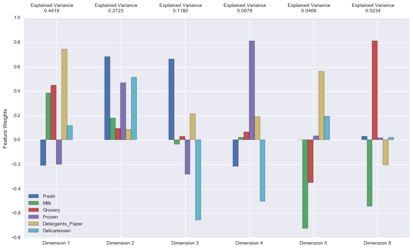
[+] How much variance in the data is explained in total by the first and second principal component?
0.7142 (71.42%) variance is explained by the 1st and 2nd PCA Dimension. Note that the 1st component is mainly driven by ‘Detergent_papers’ feature and to a lesser extent by the ‘Milk’ and ‘Grocery’ features. The 2nd PCA dimension is dominated by the triplet: ‘Fresh’, ‘Frozen’ and ‘Delicatessen’ features. The 4 first PCA Dimensions have total explained variance of more than 0.9300. Therefore, using the first 4 components is enough to capture most of the variance of the original data, i.e the dataset can be compressed from 6 dimensions (features) to 4 dimensions without loosing much information. The dimensions of the PCA represent different spending patterns, and are defined by a weighted sum of the original features. For example:
PCA_Dimension1 = 0.78 * ‘Detergents_Paper’ + 0.5 * ‘Grocery’ + 0.4 * ‘Milk’ - 0.2 * ‘Frozen’ - 0.2 * ‘Fresh’ + 0.2 * ‘Delicatessen’.
PCA_Dimension1 represents a spending pattern with higher spending on ‘Detergents_Paper’, ‘Milk’, ‘Grocery’ and ‘Delicatessen’ and decreasing spending on ‘Frozen’ and ‘Fresh’ products. PCA_Dimension1 is mostly correlated ( positively) to ‘Detergents_Paper’.
PCA_Dimension2: all product categories show positive weights but of different amplitudes, and the highest weight being for ‘Fresh’ and lowest rate for ‘Detergents_paper’.
PCA_Dimension3: is mainly correlated to ‘Delicatessen’ (negative correlation) and ‘Fresh’ (positive correlation). It reflects the case where customers who buy more ‘Fresh’ products, would consequently spend less on ‘Delicatessen’ and ‘Frozen’ products.
PCA_Dimension4: is mainly correlated to ‘Frozen’ (positive correlation) and negatively correlated to ‘Delicatessen’ and ‘Fresh’.
| Dimension 1 | Dimension 2 | Dimension 3 | Dimension 4 | Dimension 5 | Dimension 6 | |
|---|---|---|---|---|---|---|
| 0 | 1.1367 | -0.1357 | 1.2913 | -0.6126 | 0.4993 | 0.0965 |
| 1 | -3.3629 | -1.7125 | 0.3371 | 0.7769 | 0.3800 | 0.6531 |
| 2 | 1.5088 | 1.3272 | 0.5133 | -0.4019 | 0.2411 | 0.0286 |
#Dimensionality Reduction When using principal component analysis, one of the main goals is to reduce the dimensionality of the data — in effect, reducing the complexity of the problem. Dimensionality reduction comes at a cost: Fewer dimensions used implies less of the total variance in the data is being explained. Because of this, the cumulative explained variance ratio is extremely important for knowing how many dimensions are necessary for the problem. Additionally, if a signifiant amount of variance is explained by only two or three dimensions, the reduced data can be visualized afterwards.
| Dimension 1 | Dimension 2 | |
|---|---|---|
| 0 | 1.1367 | -0.1357 |
| 1 | -3.3629 | -1.7125 |
| 2 | 1.5088 | 1.3272 |
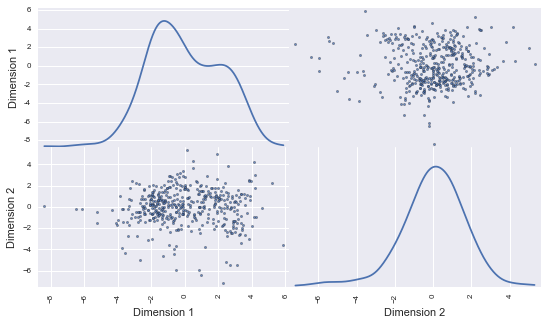
Above, the scatter matrix is plotted for Dimension1 and Dimension2. Note that Dimension1 shows a bimodal distribution. This is not unexpected: indeed, Dimension1 gets contributions mainly from ‘Milk’, ‘Grocery’ and ‘Detergents_Paper’ products (the highest weights). And we have seen earlier in this report, that the 2 features ‘Grocery and ‘Detergents_Paper’ are positively correlated. In contrast, Dimension2 shows a unimodal distribution: in this case, the main contributing features are ‘Fresh’, ‘Frozen’, and ‘Delicatessen’. Those features are uncorrelated.
Clustering
In this section, we will choose to use either a K-Means clustering algorithm or a Gaussian Mixture Model clustering algorithm to identify the various customer segments hidden in the data.
[+] K-means clustering is one of the simplest algorithm for unsupervised learning. It is fast and scale well with large dataset. Another advantage of the K-means clustering algorithm is that it makes no assumption on the distribution of the observations, and performed a hard assignment of the points to a cluster.
[+] The Gaussian Mixture Model (GMM) compute to what degree (probability) a data point is assigned to a cluster: GMM offers the possibility to relax the assignment threshold depending on the data.
We will use the GMM algorithm for the following reasons:
- with the Log transformation, the data is closer to a normal distribution: we can see uni-modal and bi-modal distribution of some features (ref. to the scatter matrix of the Log transformed features)
- our dataset is relatively small, so compute time is not an issue.
#Creating Clusters Depending on the problem, the number of clusters that we expect to be in the data may already be known. When the number of clusters is not known a priori, there is no guarantee that a given number of clusters best segments the data, since it is unclear what structure exists in the data — if any. However, we can quantify the “goodness” of a clustering by calculating each data point’s silhouette coefficient. The silhouette coefficient for a data point measures how similar it is to its assigned cluster from -1 (dissimilar) to 1 (similar).
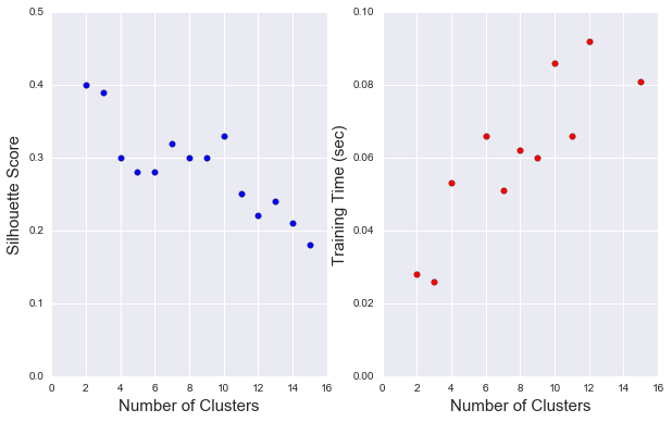
We report the silhouette score for several cluster numbers we tried.
| Nbr of clusters | silhouette score |
|---|---|
| 2 | 0.4 |
| 3 | 0.39 |
| 4 | 0.3 |
| 5 | 0.28 |
| 6 | 0.28 |
| 7 | 0.32 |
| 8 | 0.3 |
| 9 | 0.3 |
</div>
[+] The best score is obtained when using 2 clusters. However, there is not much difference between the silhouette score when using 2 clusters or 3 clusters. Beyond 3 clusters, the silouette score drops significantly.
Cluster Visualization
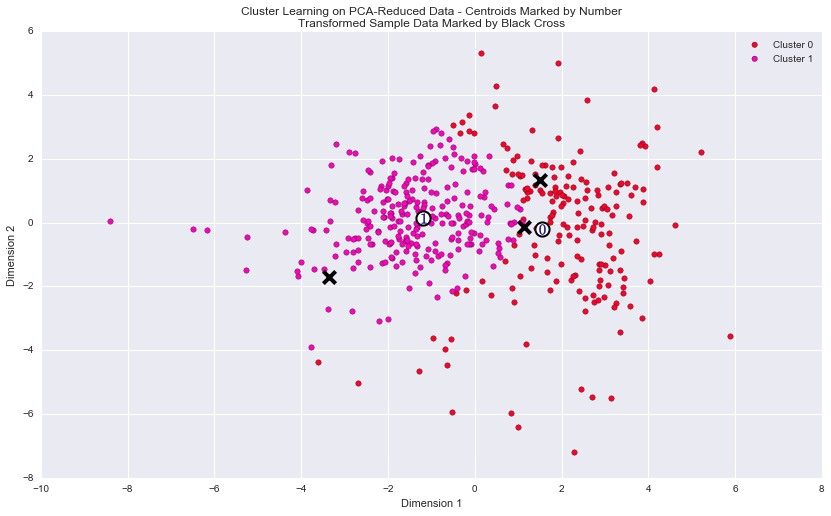
Each cluster present in the visualization above has a central point. These centers (or means) are not specifically data points from the data, but rather the averages of all the data points predicted in the respective clusters. For the problem of creating customer segments, a cluster’s center point corresponds to the average customer of that segment. Since the data is currently reduced in dimension and scaled by a logarithm, we can recover the representative customer spending from these data points by applying the inverse transformations.
| Fresh | Milk | Grocery | Frozen | Detergents_Paper | Delicatessen | |
|---|---|---|---|---|---|---|
| Segment 0 | 3920.0 | 5954.0 | 9243.0 | 989.0 | 2806.0 | 861.0 |
| Segment 1 | 8846.0 | 2214.0 | 2777.0 | 2042.0 | 375.0 | 744.0 |
[+] What set of establishments could each of the customer segments represent?
| Fresh | Milk | Grocery | Frozen | Detergents_Paper | Delicatessen | |
|---|---|---|---|---|---|---|
| Segment 0 | -4584.0 | 2327.0 | 4487.0 | -537.0 | 1990.0 | -105.0 |
| Segment 1 | 342.0 | -1413.0 | -1979.0 | 516.0 | -441.0 | -222.0 |
The segment0 spends much less on ‘Fresh’, ‘Frozen’ and ‘Delicatessen’ products compared to the median and the mean customer. In contrast spending on ‘Grocery’, ‘Milk’ is higher. This customer segment could represent Grocery stores. The segment1 spends less on ‘Milk’ ‘Grocery’ and ‘Detergents_paper’ products than the median: this segment might represent Restaurant.
Another way to look at the data is to compute the normalized spending for each segment i.e: \begin{align} \%cost = \frac{\text{feature spending}}{\text{total spending}} \end{align}
| total cost | %cost_Fresh | %cost_Milk | %cost_Grocery | %cost_Frozen | %cost_Detergents_Paper | %cost_Delicatessen | ||
| segment 0 | 23773 | 16.5 | 25.0 | 38.9 | 4.2 | 11.8 | 3.6 | |
|---|---|---|---|---|---|---|---|---|
| segment 1 | 16998 | 52.0 | 13 | 16.3 | 12.0 | 2.2 | 4.4 |
[+] segment_0: ‘Grocery’ represents the largest spending followed by ‘Milk’, ‘Fresh’ and ‘Detergents_paper’. This could represent the purchasing pattern of a Retailer.
[+] segment_1: ‘Fresh’ represents the largest spending by far, followed prractically evenly by ‘Milk’, ‘Grocery’ and ‘Frozen’. This could represent the purchasing pattern of a Restaurant.
[+] For each sample point, which customer segment best represents it?
| Customer | total cost | %cost_Fresh | %cost_Milk | %cost_Grocery | %cost_Frozen | %cost_Detergents_Paper | %cost_Delicatessen | |
| 0 | 26465 | 45.8 | 12.1 | 26.4 | 1.8 | 11.9 | 2.1 | |
|---|---|---|---|---|---|---|---|---|
| 1 | 8434 | 49.3 | 4.4 | 16.5 | 27.3 | 1.0 | 1.5 | |
| 2 | 39888 | 43.5 | 15.5 | 24.3 | 3.2 | 9.1 | 4.3 |
[+] sample_0 and sample_2 are best represented by segment_0 as their purchasing pattern better match segment_0. Although those two samples show higher %cost of ‘Fresh’ products, they also show lowest %cost for ‘Delicatessen’ and ‘Frozen’ similarly to segment_0.
[+] sample_2 purchasing pattern matches better segment_1 where the lowest %cost are for ‘Delicatessen’ and ‘Detergents_paper’.
The model predictions for each sample confirm our conclusion above. Note that in a earlier section of the assignment, we argued that sample_0 and sample_2 are likely in the same core business because of their similar purchasing pattern, and it is also confirmed by the model.
#Conclusion
[+] Companies will often run A/B tests when making small changes to their products or services to determine whether making that change will affect its customers positively or negatively. If the wholesale distributor is considering changing its delivery service for example from currently 5 days a week to 3 days a week, is that going to affect the business?
A higher frequency of delivery is likely to positively affect the customers that purchase mainly ‘Fresh’ and ‘Milk’ products. It might have no effect on other customers, although a higher frequency of truck delivery could be a disturbance (more traffic, etc..) and impact the customer’ bottom line. In order to determine which customers would respond positively to new delivery service, one could split the customers in 2 similar sets (setA and setB): i.e customers belonging to segment_0 would be equaly split between setA and setB, and same thing for customers of segment_1.
We would then expose only one set (for example setA) to the new delivery service, and keep the service unchanged for the 2nd set of customers setB.
We can then compare setA and setB to determine what group of customers that the new service affects the most.
[+]Additional structure is derived from originally unlabeled data when using clustering techniques. Since each customer has a customer segment it best identifies with (depending on the clustering algorithm applied), we can consider ‘customer segment’ as an engineered feature for the data. If the wholesale distributor recently acquired ten new customers and each provided estimates for anticipated annual spending of each product category. Knowing these estimates, the wholesale distributor wants to classify each new customer to a customer segment to determine the most appropriate delivery service. How can the wholesale distributor label the new customers using only their estimated product spending and the customer segment data?
The target variable would be the customer_segment. We could train a Decision Tree Classifier (or any other classification algorithm) on existing customers using the customer_segment as the label. The wholesale distributor can then ‘run’ the new customers through the classifier which would then outputs the segment that the new customers belong to.
Let ‘s Visualize Underlying Distributions:
At the beginning of this project, it was discussed that the 'Channel' and 'Region' features would be excluded from the dataset so that the customer product categories were emphasized in the analysis. By reintroducing the 'Channel' feature to the dataset, an interesting structure emerges when considering the same PCA dimensionality reduction applied earlier to the original dataset. We can see how each data point is labeled either 'HoReCa' (Hotel/Restaurant/Cafe) or 'Retail' the reduced space.
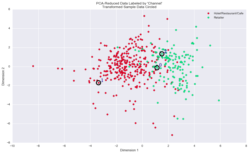
The clustering model with 2 clusters reproduces fairly well the distribution of Hotel/Restaurant/Cafe and Retailer customer. Though, there are a few data points (green) that are embedded in a large population of red data points. Our GMM model shows a clearer/sharper boundary between the 2 segments. The customers with Dimension2 in the range [-2, 2] and Dimension1 < -1 are likely to have a very high probability to belong to segment1, but there would still be a negligible probability that the customer belongs to segment0.