
As education has grown to rely more on technology, vast amounts of data has become available for examination and prediction. Logs of student activities, grades, interactions with teachers and fellow students, and more, are now captured in real time through learning management systems like Canvas and Edmodo. Within all levels of education, there exists a push to help increase the likelihood of student success, without watering down the education or engaging in behaviors that fail to improve the underlying issues. Graduation rates are often the criteria. A local school district has a goal to reach a 95% graduation rate by the end of the decade by identifying students who need intervention before they drop out of school. We will build a model that predicts how likely a student is to pass their high school final exam: **the model must be effective while using the least amount of computation costs.
Classification vs. Regression
This is a binary classification problem with a labeled dataset. Our model must output either “1” if the student passed the final exam or “0” otherwise.
Exploring the Data
Let’s begin by investigating the dataset to determine how many students we have information on, and learn about the graduation rate among these students.
[+] Total number of students: 395
[+] Number of features: 30
[+] Number of students who passed: 265
[+] Number of students who failed: 130
[+] Graduation rate of the class: 67.09%
[+] There is more Female than Male students in the dataset:
F: 208 | M: 187
[+] The number of grad Female students is about the same as that of Male students:
133 Nbr of grad Female | 132 Nbr of grad Male
[+] The Male students have a higher graduation rate: F: 0.64|M: 0.71
[+] The ratio of students attending G. Pereira versus Mousinho is 7 : 1
[+] Graduation rate at Gabriel Pereira: 0.68 | Mousinho da Silveira 0.63
[+] The graduation rate is higher for students attending Pereira: 0.05 points higher
Visualization of a few data
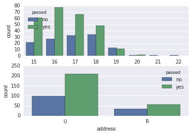
More observations: Most students with age 15 to 21 pass the final exam, with the exception of the 19 yo students (grad rate < 0.5. Note that there is only 1 student of age 21 and 1 student of age 22. There are more Urban than Rural students. The graduation rate of Urban students is higher than that of Rural Students
Preparing the Data
In this section, we will prepare the data for modeling, training and testing. It is often the case that the data you obtain contains non-numeric features. This can be a problem, as most machine learning algorithms expect numeric data to perform computations with.
[+] Feature columns
[‘school’, ‘sex’, ‘age’, ‘address’, ‘famsize’, ‘Pstatus’, ‘Medu’, ‘Fedu’, ‘Mjob’, ‘Fjob’, ‘reason’,
‘guardian’, ‘traveltime’, ‘studytime’, ‘failures’, ‘schoolsup’, ‘famsup’, ‘paid’, ‘activities’, ‘nursery’,
‘higher’, ‘internet’, ‘romantic’, ‘famrel’, ‘freetime’, ‘goout’, ‘Dalc’, ‘Walc’, ‘health’, ‘absences’]
| school | sex | age | address | famsize | Pstatus | Medu | Fedu | Mjob | Fjob | higher | internet | romantic | famrel | freetime | goout | Dalc | Walc | health | absences | |
| 0 | GP | F | 18 | U | GT3 | A | 4 | 4 | at_home | teacher | yes | no | no | 4 | 3 | 4 | 1 | 1 | 3 | 6 |
| 1 | GP | F | 17 | U | GT3 | T | 1 | 1 | at_home | other | yes | yes | no | 5 | 3 | 3 | 1 | 1 | 3 | 4 |
| 2 | GP | F | 15 | U | LE3 | T | 1 | 1 | at_home | other | yes | yes | no | 4 | 3 | 2 | 2 | 3 | 3 | 10 |
| 3 | GP | F | 15 | U | GT3 | T | 4 | 2 | health | services | yes | yes | yes | 3 | 2 | 2 | 1 | 1 | 5 | 2 |
| 4 | GP | F | 16 | U | GT3 | T | 3 | 3 | other | other | yes | no | no | 4 | 3 | 2 | 1 | 2 | 5 | 4 |
[5 rows x 30 columns]
There are several non-numeric columns that need to be converted! Many of them are simply ‘yes’/’no’, e.g. ‘internet’. These can be reasonably converted into ‘1’/’0’ (binary) values. Other columns, like ‘Mjob’ and ‘Fjob’, have more than two values, and are known as categorical variables. The recommended way to handle such a column is to create as many columns as possible values (e.g. ‘Fjob_teacher’, ‘Fjob_other’, ‘Fjob_services’, etc.), and assign a ‘1’ to one of them and ‘0’ to all others.
These generated columns are sometimes called dummy variables, and we will use the pandas.get_dummies() function to perform this transformation.
Processed feature columns (48 total features): [‘school_GP’, ‘school_MS’, ‘sex_F’, ‘sex_M’, ‘age’, ‘address_R’, ‘address_U’, ‘famsize_GT3’, ‘famsize_LE3’, ‘Pstatus_A’, ‘Pstatus_T’, ‘Medu’, ‘Fedu’, ‘Mjob_at_home’, ‘Mjob_health’, ‘Mjob_other’, ‘Mjob_services’, ‘Mjob_teacher’, ‘Fjob_at_home’, ‘Fjob_health’, ‘Fjob_other’, ‘Fjob_services’, ‘Fjob_teacher’, ‘reason_course’, ‘reason_home’, ‘reason_other’, ‘reason_reputation’, ‘guardian_father’, ‘guardian_mother’, ‘guardian_other’, ‘traveltime’, ‘studytime’, ‘failures’, ‘schoolsup’, ‘famsup’, ‘paid’, ‘activities’, ‘nursery’, ‘higher’, ‘internet’, ‘romantic’, ‘famrel’, ‘freetime’, ‘goout’, ‘Dalc’, ‘Walc’, ‘health’, ‘absences’]
| school | sex_M | sex_F | age | address_R | address_U | famsize_GT3 | famsize_LE3 | Pstatus_A | higher | internet | romantic | famrel | freetime | goout | Dalc | Walc | health | absences | |
| 0.0 | 1.0 | 1.0 | 0.0 | 18 | 0.0 | 1.0 | 1.0 | 0.0 | 1.0 | 1.0 | 0.0 | 0.0 | 4.0 | 3.0 | 4.0 | 1.0 | 1.0 | 3.0 | 6.0 |
| 1.0 | 1.0 | 1.0 | 0.0 | 17 | 0.0 | 1.0 | 1.0 | 0.0 | 0.0 | 1.0 | 1.0 | 0.0 | 5.0 | 3.0 | 3.0 | 1.0 | 1.0 | 3.0 | 4.0 |
| 2.0 | 1.0 | 1.0 | 0.0 | 15 | 0.0 | 1.0 | 0.0 | 1.0 | 0.0 | 1.0 | 1.0 | 0.0 | 4.0 | 3.0 | 2.0 | 2.0 | 3.0 | 3.0 | 10.0 |
| 3.0 | 1. | 1.0 | 0.0 | 15.0 | 0.0 | 1.0 | 1.0 | 0.0 | 0.0 | 1.0 | 1.0 | 1.0 | 3.0 | 2.0 | 2.0 | 1.0 | 1.0 | 5.0 | 2.0 |
| 4.0 | 1.0 | 1.0 | 0.0 | 16.0 | 0.0 | 1.0 | 1.0 | 0.0 | 0.0 | 1.0 | 0.0 | 0.0 | 4.0 | 3.0 | 2.0 | 1.0 | 2.0 | 5.0 | 4.0 |
[5 rows x 48 columns]
Implementation: Training and Testing Data Split
Now, we split the data (both features and corresponding labels) into training and test sets. In the following code cell below, you will need to implement the following:
[+] Randomly shuffle and split the data (‘X_all’, ‘y_all’) into training and testing subsets.
[+] Use 300 training points (approximately 75%) and 95 testing points (approximately 25%).
[+] Set a ‘random_state’ for the function(s) you use, if provided.
[+] Store the results in ‘X_train’, ‘X_test’, ‘y_train’, and ‘y_test’.
This “dummy” model predicts that all the students passed the final exam (i.e a graduation rate of 100%).
[+] Number of True Positive: 205
[+] Number of False Positive: 95
[+] The F1-score on the training set is 0.81 and on the test set 0.77. Our supervised Learning Model must perform better if using F1-score as a metric of model performance.
The confusion matrix of the naive model for the training set is shown below (in parenthesis is the count):
| Positive predict | Negative predict | |
| Positive Truth | tp (=205) | fn (=0) |
| Negative Truth | fp(=95) | tn(=0) |
The fp are false positive, i.e the examples where the model wrongly classified the students as passing the tests.
- Recall = tp/(tp+fn) = 205/(205+0) = 1
- Precision = tp/(tp + fp) = 205/(205+95) = 0.68
The F1-score might not be the best metric to evaluate the performance of the model in our problem.
We will express F1-Score in terms of tp, tn, fp, fn instead:
The equation can be simplified to:
Let’s now look at some cases:
- Case1: fn=fp=0 (i.e no misclassification), then F1-score=1 as expected
- Case2: fn=0.5 but fp=0 i.e we have 50% of the students who passed the exam were predicted to fail the exam.
- Case3: fn=0 but fp=0.5, i.e the student that failed the exam were predicted to pass the exam.
Case2 and Case3 result in the same F1-score. However, a classifier that misclassifies failing students as graduating students can be considered to be worst than a classifier that misclassifies graduating students as failing students. We might want to use a metric that put more weights on Case3 misclassifications
Training and Evaluating Models
We choose 3 supervised learning models that are appropriate for this problem.
Boosted Decision Tree Classifier(modelA)
A Boosted Decision Tree Classifier (DTC)is a supervised learning algorithm using Ensemble method to improve the accuracy of the learning algorithm. The real-world application of Boosted DTC includes star galaxy classification, assess quality of Financial Products, diagnosis of desease, object recognition and text processing.
One of the advantages of the Boosted DTC is that it can be easily visualized and explained: given a new example, its classification can be explained by Boolean Logic. A Boosted DTC has few parameters to tune, and it requires little data preparation such as normalization of the features.
One of the disadvantages of a Boosted DTC is that if the weak learners are too complex, it can result in high variance. Typically, Boosted Decision Tree Classifiers use an ensemble of DTC of depth=1, i.e Decision Stumps.
Naive Bayes Classification (modelB)
The Naive Bayes Classification (NBC) algorithm is a classification technique based on Bayes Theorem and can be used for binary and multi-class problems. It is used in spam detection, recognizing letters from handwritten texts as well as facial analysis problems. The Naive Bayes Classifier assumes that the features are conditionally independent, that is to say that given the class variable, the value of a particular feature is unrelated to that of any other features. The NBC presents the advantage to have no tuning parameters. It is easy to implement and fast to predict classes of datasets. It is also useful for models that require transparency.
NBC performs well in the case of categorical input variables compared to numerical variables. For the later case, one needs to assume normal distribution which is a strong assumption. Another disadvantage is that: if a category that is not present in the training data is found in the test data, the model will not be able to make a prediction. The assumption of independent predictors adds to the bias of the model. NBC tends to perform poorly due to their simplicity.
Logistic Regression (modelC)
Logistic Regression is a Supervised Learning Algorithm that can be used for binary classification, but also for multi-class when applying the oneVsAll method. Logistic Regression is used in Marketing to predict customer rentention, in Finance to predit stock price, and text classification. Unlike DTC or Naive Bayes Algorithm, Logistic Regression can include interaction terms to investigate potential combined effects of the variables.
The model coefficients can be interpreted to understand the direction and strength of the relationships between the features and the class. A Logistic regression without polynomial terms can only represent linear/planar boundary. In order to represent more complex boundaries, high order feature terms are required. This comes with the disadvantage of increasing the number of features, with the risk of high variance, and also increases the computing time. Though, regularization can be used to prevent overfitting. Another disadvantage of the Logistic Regression is that it requires additional data processing such as feature normalization.
We will try out Logistic Regression because it is a simple model that can be used as a benchmark. Because we are dealing with a small dataset, we also chose to experiment with the Naive Bayes Classifier because it is a high Bias classifier. Even if the features are not entirely independent, Naive Bayes can still perform well. The Model interpretability is also an important factor in the choice of the model. Indeed, those 3 models can be interpreted by the school board and reveal correlation between the student performance and the features. Those models are also cheap and fast to compute. Finally, it is also important that the models achieve high accuracy.
Setup
We run the code cell below to initialize three helper functions which you can use for training and testing the three supervised learning models. The functions are as follows:
- “train_classifier” - takes as input a classifier and training data and fits the classifier to the data.
- “predict_labels” - takes as input a fit classifier, features, and a target labeling and makes predictions using the F1 score.
- “train_predict” - takes as input a classifier, and the training and testing data, and performs
train_clasifierandpredict_labels. - This function will report the F1 score for both the training and testing data separately.
Implementation: Model Performance Metrics
[+] model A: Decision Tree Classifier with Boosting
Training a AdaBoostClassifier using a training set size of 100. . .
Trained model in 0.0072 seconds
Total observed 64 | predicted Success 64
Made predictions in 0.0022 seconds.
F1 score for training set: 1.0000.
Total observed 60 | predicted Success 56
Made predictions in 0.0012 seconds.
F1 score for test set: 0.6552.
[+] model B: Bernouilli Naive Bayes
Training a BernoulliNB using a training set size of 100. . .
Trained model in 0.0034 seconds
Total observed 64 | predicted Success 76
Made predictions in 0.0009 seconds.
F1 score for training set: 0.8286.
Total observed 60 | predicted Success 81
Made predictions in 0.0005 seconds.
F1 score for test set: 0.7943.
[+] model C: Linear Regression
Training a LogisticRegression using a training set size of 100. . .
Trained model in 0.0026 seconds
Total observed 64 | predicted Success 70
Made predictions in 0.0003 seconds.
F1 score for training set: 0.9104.
Total observed 60 | predicted Success 67
Made predictions in 0.0005 seconds.
F1 score for test set: 0.7087.
[+] model A: Decision Tree Classifier with Boosting
Training a AdaBoostClassifier using a training set size of 200. . .
Trained model in 0.0064 seconds
Total observed 138 | predicted Success 138
Made predictions in 0.0017 seconds.
F1 score for training set: 1.0000.
Total observed 60 | predicted Success 67
Made predictions in 0.0007 seconds.
F1 score for test set: 0.7402.
[+] model B: Bernouilli Naive Bayes
Training a BernoulliNB using a training set size of 200. . .
Trained model in 0.0015 seconds
Total observed 138 | predicted Success 162
Made predictions in 0.0016 seconds.
F1 score for training set: 0.8267.
Total observed 60 | predicted Success 76
Made predictions in 0.0017 seconds.
F1 score for test set: 0.7794.
[+] model C: Linear Regression
Training a LogisticRegression using a training set size of 200. . .
Trained model in 0.0091 seconds
Total observed 138 | predicted Success 147
Made predictions in 0.0008 seconds.
F1 score for training set: 0.8421.
Total observed 60 | predicted Success 77
Made predictions in 0.0003 seconds.
F1 score for test set: 0.7883.
[+] model A: Decision Tree Classifier with Boosting
Training a AdaBoostClassifier using a training set size of 300. . .
Trained model in 0.0034 seconds
Total observed 205 | predicted Success 205
Made predictions in 0.0010 seconds.
F1 score for training set: 1.0000.
Total observed 60 | predicted Success 58
Made predictions in 0.0005 seconds.
F1 score for test set: 0.6102.
[+] model B: Bernouilli Naive Bayes
Training a BernoulliNB using a training set size of 300. . .
Trained model in 0.0025 seconds
Total observed 205 | predicted Success 228
Made predictions in 0.0019 seconds.
F1 score for training set: 0.8037.
Total observed 60 | predicted Success 75
Made predictions in 0.0007 seconds.
F1 score for test set: 0.7556.
[+] model C: Linear Regression
Training a LogisticRegression using a training set size of 300. . .
Trained model in 0.0120 seconds
Total observed 205 | predicted Success 236
Made predictions in 0.0028 seconds.
F1 score for training set: 0.8435.
Total observed 60 | predicted Success 73
Made predictions in 0.0007 seconds.
F1 score for test set: 0.7820.
Tabular Results
** Classifer 1 - Decision Tree Classifier **
| Training Set Size | Prediction Time (test) | Training Time | F1 Score (train) | F1 Score (test) |
| 100 | 0.0059406 | 0.0006511 | 1.0 | 0.6207 |
| 200 | 0.0061325 | 0.0005101 | 1.0 | 0.7360 |
| 300 | 0.0065699 | 0.0005306 | 1.0 | 0.6281 |
** Classifer 2 - Naive Bayes **
| Training Set Size | Prediction Time (test) | Training Time | F1 Score (train) | F1 Score (test) |
| 100 | 0.001072 | 0.0004 | 0.8206 | 0.7943 |
| 200 | 0.001585 | 0.0007 | 0.8267 | 0.7794 |
| 300 | 0.001323 | 0.0004 | 0.8037 | 0.7556 |
** Classifer 3 - Logistic Regression**
| Training Set Size | Prediction Time (test) | Training Time | F1 Score (train) | F1 Score (test) |
| 100 | 0.002504 | 0.000122 | 0.9104 | 0.7087 |
| 200 | 0.002925 | 0.000122 | 0.8421 | 0.7883 |
| 300 | 0.003895 | 0.000122 | 0.8435 | 0.7820 |
The Boosted Decision Tree Classifier (DTC) is the best performing model, although it is the slowest of the 3 models. The Boosted DTC when using the default settings does not perform better than the Naive Bayes nor the Logistic Regression Classifier. However, the settings can be tweaked (as it will be done later) in order to improve the performance. In particular, it is clear that, as is (i.e with the default settings), our Boosted DTC suffers from overfitting as demonstrated by a F1-score=1 for the training set (300 examples), and a poor F1-score of 0.63 for the test set.
The goal of the model is to predict whether a student will pass the final exam. In order to build our model, we take a sample of students whose the result at the final exam is known. Each student is “defined” by a set of characteristics/attributes: gender, address, the school attended, etc…
The model consists in generating a number of simple rules on the students attributes, with a classification error below better than 0.5, i.e better than . For example, one possible rule could be to split the students depending on the area: Urban or Rural. If all the students with the Urban attribute had passed the exam, and all the students with Rural attribute had failed, then this rule alone would be sufficient to classify students, and predict outcome for future students. But such a simple rule is very likely to make errors. A new rule is then generated and it will pay more attention to the examples that were misclassified by the previous rule. As new rules are generated, they will continue to pay more attention to the examples that have been misclassified by the preceding rule.
After many iterations of generating new rules, the prediction from all those simple rules are combined in the form of a weighted average, which will have much more accuracy than the prediction from a single rule alone.
Implementation: Model Tuning
The final model has a F1-score of 0.82 for the training set and 0.80 for the test set. The F1-score of training set is lower for the tuned model: 0.82 versus 1.0 for the untuned model. And the F1-score of the test set is improved after tuning the model. The results clearly indicate that there is less overfitting in the tuned model. Indeed, ($\Delta$ F1-score), i.e “F1-score of training set” minus “F1-score of test set”, is lower for the tuned model.