
In this project, we analyze the prices of homes in suburbs of Boston. We build a predictive model and train/test it on collected data. The performance of the model is then evaluated. The model can then be used to make certain predictions about a home — in particular, its monetary value. This model would prove to be invaluable for someone like a real estate agent who could make use of such information on a daily basis.
The dataset for this project originates from the UCI Machine Learning Repository. The Boston housing data was collected in 1978 and each of the 506 entries represent aggregated data about 14 features for homes from various suburbs in Boston, Massachusetts. For the purposes of this project, the following pre-processing steps have been performed on the dataset:
[+] 16 data points have an “MDEV” value of 50.0. These data points likely contain missing or censored values and have been removed.
[+] 1 data point has an “RM” value of 8.78. This data point can be considered an outlier and has been removed.
[+] The features “RM”, “LSTAT”, “PTRATIO”, and “MDEV” are essential. The remaining non-relevant features have been excluded.
[+] The feature “‘“MDEV” has been multiplicatively scaled to account for 35 years of market inflation.
Boston housing dataset has 489 data points with 4 variables each. Input size: (489, 4)
Data Exploration
First, we separate the dataset into features and the target variable. The features, “RM”, “LSTAT”, and “PTRATIO”, give us quantitative information about each data point. The target variable, “MDEV”, will be the variable we seek to predict. These are stored in ‘features’ and ‘prices’, respectively.
Implementation: Calculate Statistics
We report descriptive statistics about the Boston housing prices.
Statistics for Boston housing dataset:
Minimum price: $105,000.00
Maximum price: $1,024,800.00
Mean price: $454,342.94
Median price $438,900.00
Standard deviation of prices: $165,171.13
Feature Observation
We are using three features from the Boston housing dataset: “RM”, “LSTAT”, and “PTRATIO”. For each data point (neighborhood):
[+] “RM” is the average number of rooms among homes in the neighborhood.
[+] “LSTAT” is the percentage of all Boston homeowners who have a greater net worth than homeowners in the neighborhood.
[+] “PTRATIO” is the ratio of students to teachers in primary and secondary schools in the neighborhood.
When the “RM” is high, the homes are likely to have a larger surface area, and therefore a higher “MDEV”. If “LSTAT” is low, i.e the homeowners of the neighborhood have a net worth in the top bracket of the Boston population. This is likely an upper class neighborhood therefore the “MDEV” is expected to be higher. In contrast if the “LSTAT” is high, the homeowners of the neighborhood have a net worth in the bottom bracket of the Boston population. This is likely a neighborhood with low income population, and the “MDEV” would be low. 3) “MDEV” would be inversely impacted by the “PTRATIO”: for low “PTRATIO” (higher number of teachers per students), which is typically find in good schools, the “MDEV” would likely be higher.
Developing a Model
In this second section of the project, we develop the tools and techniques necessary for a model to make a prediction. It is difficult to measure the quality of a given model without quantifying its performance over training and testing. This is typically done using some type of performance metric, whether it is through calculating some type of error, the goodness of fit, or some other useful measurement. For this project, we will be calculating the coefficient of determination, R2, to quantify our model’s performance. The coefficient of determination for a model is a useful statistic in regression analysis, as it often describes how “good” that model is at making predictions.
The values for R2 range from 0 to 1, which captures the percentage of squared correlation between the predicted and actual values of the target variable. A model with an R2 of 0 always fails to predict the target variable, whereas a model with an R2 of 1 perfectly predicts the target variable. Any value between 0 and 1 indicates what percentage of the target variable, using this model, can be explained by the features. A model can be given a negative R2 as well, which indicates that the model is no better than one that naively predicts the mean of the target variable.
Implementation: Shuffle and Split Data
Now, we will split the data into training and testing subsets. Typically, the data is also shuffled into a random order when creating the training and testing subsets to remove any bias in the ordering of the dataset.
Splitting the data into training and test subset enables to evaluate the model performance on previously unseen data (the test data): evaluate whether the model suffers from overfitting (high variance) or underfitting (high bias). If the data is not splitted, it is not possible to determine whether the model would generalized well.
Analyzing Model Performance
We take a look at several models’ learning and testing performances on various subsets of training data. Additionally, we’ll investigate one particular algorithm with an increasing max_depth parameter on the full training set to observe how model complexity affects performance.
Learning Curves
The following code cell produces four graphs for a decision tree model with different maximum depths. Each graph visualizes the learning curves of the model for both training and testing as the size of the training set is increased. Note that the shaded region of a learning curve denotes the uncertainty of that curve (measured as the standard deviation). The model is scored on both the training and testing sets using R2, the coefficient of determination.
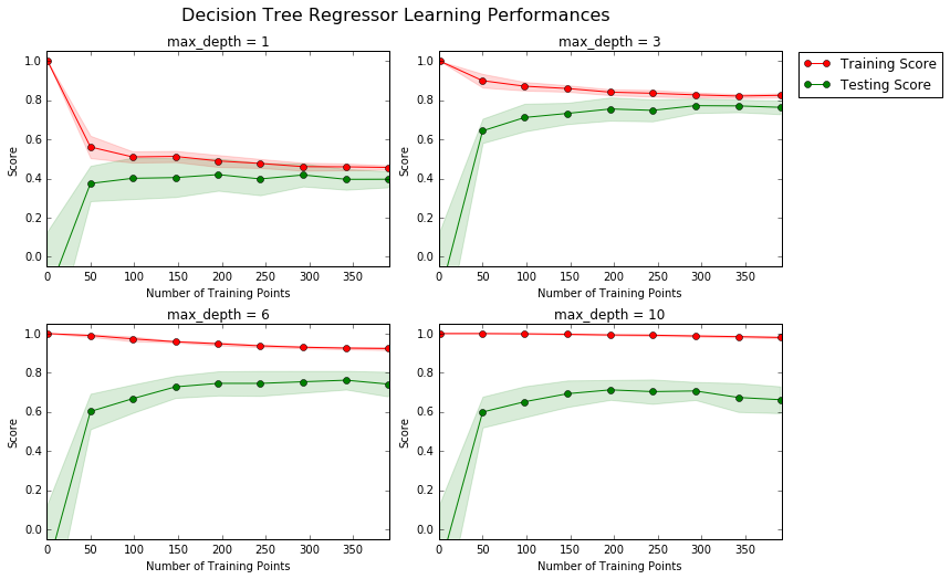
Learning the Data
The maximum_depth for the selected model is 6. With increasing the number of training points, the score of the training set decreases from 1.0 to 0.9. For training points larger than 300, the score of the training set is practically constant. With increasing the number of points, the model is finding more difficult to fit all the data points, hence the decrease of the training score. The test score increases with increasing number of training points. With small number of training points, the model suffers from overfitting and fail to gneeralize to the test data. The model will not benefit from having more training points, as both training and test score show convergence for training points above 300.
Bias-Variance Tradeoff
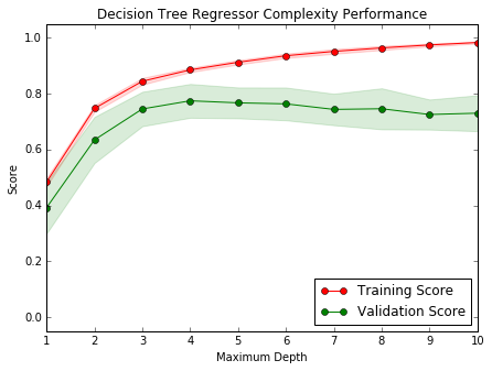
When the model is trained with a maximum depth of 1, the model suffer from high bias: the score on both the training set and the validation set is low: ~50%. With a maximum depth of 10, the model suffers from high variance: the training score is high but the validation score is lower. A maximum depth of 4 is optimum as it gives a large training score and a maximum score for the validation set.
Evaluating Model Performance
Grid Search
The grid search technique uses a range of values for the hyper-parameters like the max_depth in order to find the optimum hyper-parameters values that result in the best performing model.
Cross-Validation
In k-fold cross-validation, the original sample is randomly partitioned into k equal sized subsamples. One subsample is used as the validation set for testing the model, and the remaining (k − 1) subsamples are used as training data. The cross-validation process is then repeated k times, with each of the k subsamples used exactly once as the validation data. The k results are then averaged to produce a single estimation. The k-fold cross-validation gives better accuracy than regular train/test split. When the number of samples is low, it is prefered to use k-fold cross validation training technique with the grid-search
Fitting a Model
Parameter max_depth is 4 for the optimal model.
Example
Imagine now that we were a real estate agent in the Boston area looking to use this model to help price homes owned by your clients that they wish to sell. We have collected the following information from three of our clients:
| Feature | Client 1 | Client 2 | Client 3 |
| Total number of rooms in home | 5 rooms | 4 rooms | 8 rooms |
| Household net worth (income) | Top 34th percent | Bottom 45th percent | Top 7th percent |
| Student-teacher ratio of nearby schools | 15-to-1 | 22-to-1 | 12-to-1 |
[+] Predicted selling price for Client 1’s home: $324,240.00
[+] Predicted selling price for Client 2’s home: $189,123.53
[+] Predicted selling price for Client 3’s home: $942,666.67
The predicted selling prices are in the same range than the training data: price for Client2 is close to the minimum value of the training data, price of client close to the median, and the price for Client3 is close to the maximum price of the training data. As expected Client3 with higher number of rooms, in a upper class neighborhood and lower student-teacher ratio. The home of client2 in a neighborhood with the highest student-teacher ratio and small number of rooms and lower net worth is accurately predicted to have the lowest price.
Sensitivity
An optimal model is not necessarily a robust model. Sometimes, a model is either too complex or too simple to sufficiently generalize to new data. Sometimes, a model could use a learning algorithm that is not appropriate for the structure of the data given. Other times, the data itself could be too noisy or contain too few samples to allow a model to adequately capture the target variable — i.e., the model is underfitted. We run the code cell below to run the fit_model function ten times with different training and testing sets to see how the prediction for a specific client changes with the data it’s trained on.
[+] Trial 1: $324,240.00
[+] Trial 2: $324,450.00
[+] Trial 3: $346,500.00
[+] Trial 4: $420,622.22
[+] Trial 5: $302,400.00
[+] Trial 6: $411,931.58
[+] Trial 7: $344,750.00
[+] Trial 8: $407,232.00
[+] Trial 9: $352,315.38
[+] Trial 10: $316,890.00
Range in prices: $118,222.22
Applicability
1) How relevant today is data that was collected from 1978?
Although the price data was adjusted to account for inflation, other factors can impact housing prices: national economy (slow down or growing economy), unemployement rate, income growth rate. Therefore, the data collected from 1978 is not relevant today.
2) Are the features present in the data sufficient to describe a home?
Other features can impact the price of the house: square footage (house + low), aminities (pool, deck, patio, garage), age of the house… The features present in the data are not sufficient to describe a home.
3) Is the model robust enough to make consistent predictions?
The model is not robust enough as shown by the output above: where the predicted prices for a specific client would changed by up to $118222.22. It represents 33% of the mean predicted price.
4) Would data collected in an urban city like Boston be applicable in a rural city?
No.
The constructed model should not be used in a real-world setting.